


Continuous Improvement in Roll Forming
Can you find your hidden roll formers? They are on your plant floor, but not necessarily in plain sight. Most roll formers produce at a rate far below their true potential. Rather than seek out this hidden capacity, many companies simply purchase more machines and expand their facilities. While this approach certainly works, it may not be the best use of the company’s resources. A 1999 study by Rohm and Haas Corporation determined that developing the capacity of existing equipment and facilities was ten times less expensive than building new capacity. [1]
By using a simple performance metric, Overall Equipment Effectiveness (OEE), and by embracing the concept of continuous improvement, you can dramatically enhance the productivity, quality, and reliability of your operation.
This paper serves as an introduction to some key concepts in the field of continuous productivity and quality improvement:
Continuous improvement methodologies
- OEE measurements
- Commonly used analysis and improvement techniques
- While each of these topics will be discussed in this paper, more in-depth resources on these subjects can be found in the bibliography.
Continuous Improvement Methodologies
Continuous improvement is the ongoing improvement of products, processes, and services through incremental and radical steps.
There are a number of different approaches to continuous improvement. Each system has unique aspects and different emphasis, but all share the same basic assumptions: an organization has limited capital and management time, and these resources should be put to the very best use in order to optimize productivity and quality. Improvement efforts are cyclical and never ending.
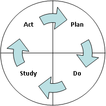
Demming Cycle
The Demming cycle was originally conceived by Walter Shewhart in the 1930s. It was later popularized by W. Edwards Demming and adopted by the Japanese in the 1950s (who referred to it as the Demming cycle). The approach involves the following steps:
Plan – Examine the current situation, gather data, identify problems, and develop solutions.
Do – Test out the plans on a trial basis (minimizing disruption) and collect resulting data.
Study/Check – Determine whether or not the plan achieved the desired results. Modify the plan if needed.
Act – Implement the plan throughout the organization.
DMAIC
The American Society for Quality defines DMAIC as “a data-driven quality strategy for improving processes and an integral part of a Six Sigma quality initiative.” [2] DMAIC is an acronym for the following steps:
- Define – Clearly define the problem to be solved. Define the current state as well as the expected results after the improvement project.
- Measure – Define the questions to be answered, what form the answers will be in, where the data will come from, and how to collect the information with minimal effort and lowest chance of errors.
- Analyze – Focus on why defects or errors occur. Identify the root causes of the problem. Conduct experiments to confirm hypotheses in a statistically valid form.
- Improve – Generate multiple solutions via brainstorming. Evaluate each idea and select the most promising solution. Confirm the success of the solution relative to the expected results; refine if necessary.
- Control – Put a system in place to maintain the results. Establish necessary policies, procedures, and training. Develop controls to ensure that key variables remain within the acceptable range.
FADE
The FADE model is similar to the Demming and DMAIC systems and is widely used in healthcare and many branches of the government. FADE stands for:
- Focus – Select a problem to be addressed, characterize the current process, show why a change is necessary, and describe the desired end result and the benefits of the change.
- Analyze – Describe the process in greater detail, develop root causes, and identify what information is necessary.
- Develop – Create a solution and implementation plan with financial justification.
- Execute – Implement the solution and establish a monitoring plan.
In each of these systems, the same basic themes are repeated. Continuous improvement is a process of optimization. A company must find the most efficient method of identifying problems, finding root causes, developing and validating solutions, and implementing the solutions in a sustainable fashion. When one project comes to a successful conclusion, the process starts over with the next most pressing issue.
One of the keys to monitoring performance and identifying problem areas is the regular review of a few key performance metrics.
Measuring Performance and Capacity – OEE and TEEP
Overall Equipment Effectiveness (OEE) is a measurement of how effectively a machine is operating during the time it is scheduled to run. OEE is used as a primary performance metric and was developed as part of the Total Productive Maintenance (TPM) process.
There are three main components of OEE:
- Availability – The ratio of machine run time to the scheduled production time.
- Speed – The ratio of actual running speed to the machines maximum speed.
- Yield – The ratio of good material produced to the total material used.
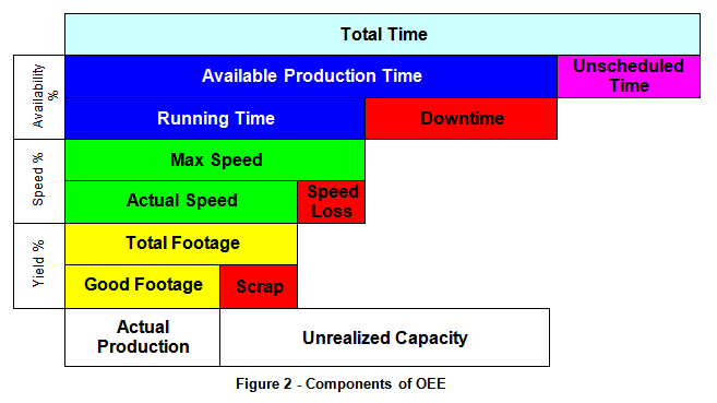
Each of these components is expressed as a percentage, and the product of all three is the OEE value. A shift OEE of 100% would require that a machine run an entire shift (less break times) with no downtime, at the maximum rated speed, and with no scrap. Although there may be single-profile tube mills with coil accumulators that might approach 100% OEE, most roll formers are running somewhere between 20% and 65% OEE.
It is important to note that unscheduled time is not considered in the availability percentage. Unscheduled or exempt time includes all break times, meetings, planned maintenance, training time, and other intentional breaks in production. These downtimes do not affect the OEE metric. They do, however, affect the Total Effective Equipment Performance (TEEP) calculation.
The three components of OEE: availability, speed, and yield, can be further broken into sub-categories:
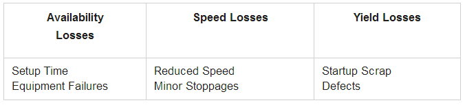
When reviewing setup time on roll forming machines, it may be helpful to consider the limits of the equipment, the performance of the operator within those limits, and the efficiency of the production schedule. Coil changes and profile changeovers are a natural part of roll forming. Some machines are designed to minimize the downtime associated with these operations and some are not. The operator should be evaluated on how well he or she is able to work within the constraints of the equipment. The last area that could affect the amount of machine setup-related downtime is the production schedule itself. Changing over to the same profile or material multiple times in a short period of time because of a lack of planning is just as wasteful as poor operator or equipment performance.
Minor stoppages (short stops) are simply delays that are too brief to be worth recording. On machines with automated downtime recording, losses due to short delays can be handled as another availability loss.
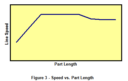
In general, the speed rate is calculated based on the number of parts produced while the machine is running. With roll forming, however, it may be more helpful to consider the average running speed of the machine in feet-per-minute (FPM). Unfortunately, using a part rate or average FPM does not provide an honest measurement of performance. Roll formers may have different maximum speeds depending on the product and part length being run at the time. Press stroke rates may limit the maximum line speed when running short parts. Handling problems may limit the speed when running very long parts. Figure 3 illustrates the relationship between maximum speed and part length found on many roll formers:
In cases where the roll former is feeding parts into a lean manufacturing cell, the running speed may be reduced to correspond to the takt time of the cell. Takt time (typically expressed in seconds) is the heartbeat of a lean manufacturing operation and is defined as the available production time divided by the customer demand for that period. The maximum speed used to calculate the speed % should be then based on the takt time rate.
The following is an example of an OEE calculation for a roll former. In an eight hour shift, there was a total of one hour break time (30 minute lunch and two fifteen minute coffee breaks). The machine ran a total of 153 minutes. There were a number of downtime occurrences:
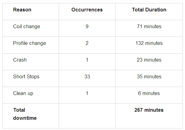
While the machine was running, it ran at an average rate of 483 FPM. The roll former is capable of running at 525 FPM average for the profiles and lengths run during the shift. Of the 74,000 feet of material run on the machine, 216 feet were considered scrap.
OEE % = Availability % × Speed % × Yield %
Availability % = (Run Time)/(Available Time) = (153 min)/(420 min) = 36%
Speed % = (Actual Rate)/(Max Rate) = (483 fpm)/(525 fpm) = 92%
Yield % = (Good Footage)/(Total Footage) = (73,784 ft)/(74,000 ft) = 99%
OEE % = 0.36 × 0.92 × 0.99 = 33%
It’s important to note that the available time does not include the total shift time. Since the machine was not expected to run during the lunch and breaks, this unscheduled time must be considered exempt from the availability calculation.
Is an OEE of 33% a good value? The answer depends on the type of equipment and the nature of the product being produced. The most important use of the OEE metric is in the monitoring of machine effectiveness over time.
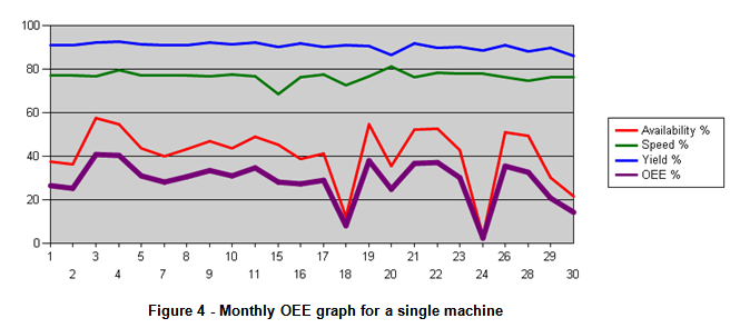
Provided that the methods of measurement remain consistent, OEE becomes the yardstick used to gauge the overall effectiveness of changes implemented in a continuous improvement cycle.
TEEP
Total Effective Equipment Performance, or TEEP, is very similar to the OEE metric, except it considers the total clock or calendar time available to run production and not just the scheduled production time. For an operation that runs two eight-hour shifts, the OEE metric considers only the 16 hours minus scheduled downtimes as available production time. TEEP includes all 24 hours and is a more direct measurement of the possible capacity of the equipment.
TEEP % = Asset Utilization % × Speed % × Yield %
Asset Utilization % = (Run Time)/(Total Time) = (153 min)/(1440 min) = 11%
Speed % = (Actual Rate)/(Max Rate) = (483 fpm)/(525 fpm) = 92%
Yield % = (Good Footage)/(Total Footage) = (73,784 ft)/(74,000 ft) = 99%
TEEP % = 0.11 × 0.92 × 0.99 = 10%
Analysis Tools
There are a number of methods available to help decide where best to focus improvement efforts and spending.
The Five Why Method
The Five Why technique is a useful way to determine the root cause of a particular problem. Rather than stop at the first cause of a defect or problem, the reason for that cause is questioned with successive research into each reason and cause, until the root cause is discovered. It is not necessary to stop after exactly five “whys” have been asked, only that the questions continue until the underlying cause is discovered.
For example, a roll former with a post-cut shear crashed and sent material up into the rafters. Why did the material buckle up? Because it jammed in the shear die during the cut. Why did the material jam in the shear die? Because the die was dull. Why was the die dull? Because it was missed the last sharpening rotation. Why did it miss the rotation? Because of poor record keeping. The process continues for as many whys as necessary to get to the root cause.
Cause and Effect Diagrams
When investigating production problems, it is important to analyze the various causes responsible for a particular effect. Fishbone (Ishikawa) diagrams can be used to identify the various causes and contributing issues. While these diagrams do not necessarily indicate the relative magnitude of each cause, they do help limit the scope of subsequent data collection efforts.
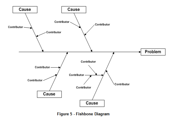
Fishbone diagrams are best developed in a brainstorming setting with people directly involved in the process. Each branch off the main problem line represents a potential cause leading to the problem. Additional contributing factors are also shown for each branch.
Pareto Analysis
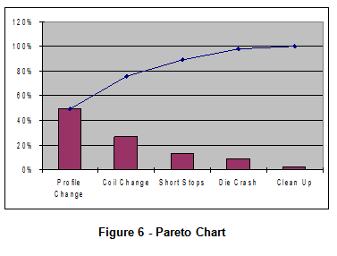
A pareto chart is a histogram of items sorted by descending frequency. It often shows that a high percentage of problems (downtime, slowdowns, and defects) are caused by only a few issues. Concentrating efforts to improve the left-most issues will result in the most dramatic results for the time and money invested.
Figure 6 shows a portion of a pareto chart of downtime reasons for single machine for a month of production. The height of the bar indicates the percentage of total downtime for each delay reason. It can also be helpful to include a plot of cumulative percentages. This can show that the top few issues make up a significant percentage of the total problems. For example, Figure 6 shows that approximately 75% of the total downtime was a result of profile or coil changes.
Pareto charts may be used in a progressive fashion to drive down through more levels of detail. In the example given, the next step may to create a pareto chart for coil change delays categorized by operator, material, or product. This may indicate specific problem areas that should be addressed first.
SPC Tools
Although a full discussion of statistical process control (SPC) falls outside the scope of this document, it may be useful to consider two aspects of SPC when dealing with defect rates in a process. It is important to determine whether or not the equipment in question is capable of reliably producing to within the required tolerance and whether or not the process is in control.
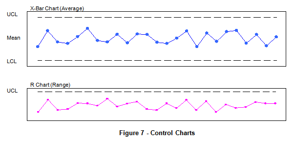
Before determining the capability of the equipment, it is first necessary to make sure it is in statistical control. This is done through the use of control charts (x-bar and R charts). These charts are based on samples of 5 consecutive parts taken on a regular time base (every 15 minutes, 30 minutes, hour, etc). The x-bar chart shows the average value of the five measurements. The R chart shows the range for each sample. The data being plotted is for a particular attribute of the part (i.e., length). Because there may be various nominal values for the attribute in question, the calculation of the average and range is based on the error (the difference between nominal and measured values). With both types of charts it is necessary to calculate control limits to be used when determining if the process is in control.
The R chart should be analyzed first, since there some special cases where particular patterns in the R chart can skew the pattern in the x-bar chart. When using a five data-point sample, the lower control limit on the R chart is zero. All data points should be within the control limits and no unusual pattern should exist (consult a text on SPC for a description of what is considered unusual). The following are general guidelines for determining control:
- No points are outside the control limits.
- The number of points above and below the center line is about the same.
- The points seem to fall randomly above and below the centerline.
- Most points, but not all, are near the center line, and only a few are close to the control limits. [3]
Once the process is determined to be in statistical control, the next step is to find out if the equipment is capable of reliably producing to within the required tolerance. A sample of 25 to 100 parts of the same type should be run with a competent operator and decent material. Each part produced should then be carefully measured with a sufficiently high precision method. From this data, a number of calculations can be made to provide a few key metrics of process capability. The first of these is the Process Capability Index, CP. The process capability index relates the natural variation of the process to the specified tolerance range.
CP = (upper tolerance limit – lower tolerance limit)
6σ
Where sigma, σ, is the standard deviation of the sample.
The process capability index does not consider how centered the results were relative to the nominal value. The other commonly used capability index is C Pk, which does factor in how well the data is centered. CPk is equal to CP if the data is perfectly centered about the nominal value.
CPk = min( CPU , CPL )
Where
CPU = (upper tolerance limit – μ)
3σ
And
CPL = (μ – lower tolerance limit)
3σ
The following table shows the relationship between CPk values and the expected defect rate:
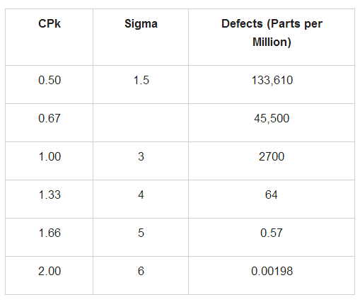
Capability studies should be performed on equipment at the beginning of an improvement project as a baseline and after any major change to verify forward progress. Control charts should be used on a regular bases (daily if possible) to monitor equipment and assure the process is still in control.
Improvement Techniques
Once problem areas are identified, the next step is to work to address them. While processes such as kaizan blitz help with general problem solving, there are two techniques that relate specifically to reducing downtime and improving quality.
Single Minute Exchange of Die (SMED)
SMED was developed by Shigeo Shingo as part of the Toyota Production System. It was designed to take machine changeovers that used to last up to several hours and improve them so they could be accomplished in less than ten minutes. Steps in a changeover can be separated into two categories: operations that can only be done with the machine stopped (internal) and those that can be performed off-line while the machine is still running (external). Recognizing the difference is critical.
The following are the three major stages of the SMED system:
- Determine exactly which steps are internal or external and make sure that only internal operations happen when the machine is stopped.
- Find ways to convert internal activities to external activities.
- Streamline all activities to reduce the changeover time. This may include involving additional staff working in parallel. The use of quick-release clamps and machine automation can help in this stage.
For a roll former with a single-mandrel uncoiler, there are a few activities that can be done in the first stage of SMED, such as preparing the new coil so that it is in close proximity to the uncoiler before the change. An upgrade to a double-mandrel uncoiler shifts the loading and unloading of the coil to be external steps. The only internal steps remaining involved the switching of the uncoiler sides and the threading of the new coil. The addition of a coil accumulator eliminates all internal steps, since the new coil is loaded and butt-welded to the previous coil while the machine is still running (the accumulator gives the operator a few minutes to complete the joining operation).
The use of rafted mills or duplex mills is another example of shifting from internal to external steps when changing profiles.
Zero Quality Control (ZQC)
Rather than spending time trying to catch defects or mistakes after they’ve occurred, ZQC encourages the fool-proof prevention of problems. This involves 100% inspections of parts at each step (an automatic check if possible), immediate feedback if problems occur, and the use of “poka-yoke” systems wherever appropriate.
The poka-yoke approach typically involves the use of simple sensors or jigs to either let the operator know immediately if something has been forgotten or improperly installed or to physically prevent mistakes to begin with. A simple example of this would be designing an electrical connector so that it can only be plugged in one way (the correct way).
Capturing the Gain
There are a number of ways to translate increased knowledge, productivity, and quality into financial gains.
Through the use of OEE and other analysis tools, manufacturers are able to optimize capital spending. In some cases, this may mean upgrades of uncoilers, mills, or press systems to improve areas that were restricting productivity. In other cases, it may still be necessary to purchase new machines, but these purchases can be made with the knowledge of what features really aid in effective production.
Improvements in efficiency can result in lower labor costs for the same output. In situations where the sales volume is fixed, reductions can be made in the number of shifts or overtime hours required. The newly created free time can also be spent improving machine reliability through autonomous maintenance or on other improvement projects.
In Overall Equipment Effectiveness, Robert Hansen describes various scenarios involving the financial impact of increased OEE. [4] In the case of fixed sales, Hansen demonstrates how a 10% increase in OEE could lead to a 21% increase in operating income and a 21% increase in return on assets (ROA). Obviously the magnitude of these improvements will vary from operation to operation. These calculations were based on labor savings at normal rates; in many cases, much of the labor savings would be at overtime rates.
In cases where the sales volume can be increased to meet the new capacity, dramatic financial gains are possible. In the same scenario, but with the factory running at full capacity due to expanded sales, Hansen shows the same 10% OEE increase led to a 62% increase in operating income and a 54% increase in ROA.
How difficult is a 10% improvement in OEE? In the example OEE calculation, a 10% increase could be accomplished by reducing the average coil change time from 7.88 minutes to 5 minutes and reducing the average profile change from 66 to 55 minutes. By contrast, to achieve the same OEE increase by simply running faster would require the mill to run an average speed of 633 FPM (20% higher than the rated speed). This example illustrates how good information is key to making effective improvements.
Anyone involved in manufacturing operations or engineering should be concerned with constantly improving productivity, quality, and reliability. The financial benefits of continuous improvement can be considerable. On the other hand, not making improvements means you are probably losing ground to your competitors.
Although this document has focused exclusively on continuous improvement in a manufacturing environment, most of the methodologies and tools described can be used throughout an organization. Continuous improvements should be applied across all areas of a company and at all levels.
Bibliography
Robert C. Hansen, Overall Equipment Effectiveness. Industrial Press, 2002.
James R. Evans and William M Lindsay, The Management and Control of Quality, 6th Edition. Thomson South-Western, 2004.
The Productivity Development Team, OEE for Operators. Productivity Press, 1999.
Joseph M. Juran, A. Blanton Godfrey, et al., Juran’s Quality Handbook, 5th Edition. McGraw-Hill, 1999.
Shigeo Shingo, A Revolution in Manufacturing: The SMED System. Productivity Press, 1985.
Shigeo Shingo, Zero Quality Control: Source Inspection and the Poka Yoke System. Productivity Press, 1986.
Peter S. Pande, Robert P. Neuman, Roland R. Cavanagh, The Six Sigma Way. McGraw-Hill, 2000.
James P. Womack and Daniel T. Jones, Lean Thinking, 2nd Revision. Free Press, 2003.
References
[1] Hansen, 19
[2] The American Society for Quality – Quality Glossary: www.asq.org/info/glossary
[3] Evans & Lindsay, 697
[4] Hansen, 48-66
